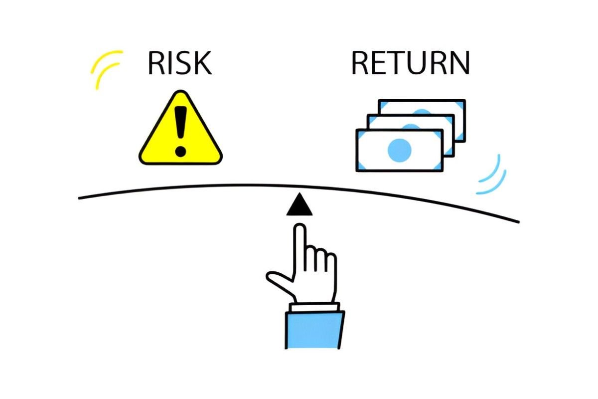
When I first started exploring the world of finance, one concept that stood out as both fundamental and fascinating was the Risk-Return Trade-Off Theory. This principle lies at the heart of nearly every financial decision, whether you’re an individual investor, a corporate treasurer, or a portfolio manager. In this article, I’ll take you through the intricacies of this theory, explain its mathematical foundations, and show you how it applies to real-world scenarios.
Table of Contents
What Is the Risk-Return Trade-Off Theory?
The Risk-Return Trade-Off Theory posits that the potential return on an investment is directly related to the level of risk associated with it. In simpler terms, higher risk typically leads to higher potential returns, while lower risk generally results in lower returns. This relationship is not just a theoretical construct; it’s a practical guide that helps investors make informed decisions.
For example, investing in government bonds is considered low-risk, but the returns are modest. On the other hand, investing in a startup company carries significant risk, but the potential for high returns is much greater. Understanding this trade-off is crucial for building a balanced portfolio that aligns with your financial goals and risk tolerance.
The Mathematical Foundation of the Risk-Return Trade-Off
To fully grasp the Risk-Return Trade-Off, we need to dive into some basic financial mathematics. Let’s start with the concept of expected return and risk.
Expected Return
The expected return of an investment is the weighted average of all possible returns, where the weights are the probabilities of each outcome. Mathematically, it can be expressed as:
E(R) = \sum_{i=1}^{n} P_i \times R_iWhere:
- E(R) is the expected return.
- P_i is the probability of the i^{th} outcome.
- R_i is the return of the i^{th} outcome.
For example, suppose you’re considering an investment with three possible outcomes:
- A 10% return with a 50% probability.
- A 5% return with a 30% probability.
- A -2% return with a 20% probability.
The expected return would be:
E(R) = (0.5 \times 0.10) + (0.3 \times 0.05) + (0.2 \times -0.02) = 0.05 + 0.015 - 0.004 = 0.061So, the expected return is 6.1%.
Risk
Risk, in financial terms, is often measured by the standard deviation of returns. Standard deviation quantifies the variability or volatility of returns around the expected return. A higher standard deviation indicates greater risk.
The formula for standard deviation is:
\sigma = \sqrt{\sum_{i=1}^{n} P_i \times (R_i - E(R))^2}Using the same example, let’s calculate the standard deviation:
- Calculate the squared deviations:
- (0.10 - 0.061)^2 = 0.001521
- (0.05 - 0.061)^2 = 0.000121
- (-0.02 - 0.061)^2 = 0.006561
- Multiply by their probabilities:
- 0.5 \times 0.001521 = 0.0007605
- 0.3 \times 0.000121 = 0.0000363
- 0.2 \times 0.006561 = 0.0013122
- Sum the results:
- 0.0007605 + 0.0000363 + 0.0013122 = 0.002109
- Take the square root:
- \sigma = \sqrt{0.002109} \approx 0.0459
So, the standard deviation is approximately 4.59%.
The Risk-Return Trade-Off in Practice
Now that we’ve covered the basics, let’s see how this theory plays out in real-world scenarios.
Example 1: Government Bonds vs. Stocks
Government bonds, such as U.S. Treasury bonds, are considered one of the safest investments. They offer a fixed interest rate and are backed by the full faith and credit of the U.S. government. However, the returns are relatively low.
On the other hand, stocks are riskier. Their prices fluctuate based on market conditions, company performance, and other factors. But historically, stocks have provided higher average returns than bonds over the long term.
Let’s compare the two:
| Investment Type | Expected Return | Standard Deviation (Risk) |
|---|---|---|
| Government Bonds | 2% | 1% |
| Stocks | 8% | 15% |
As you can see, stocks offer a higher expected return but come with significantly higher risk.
Example 2: Diversification and Portfolio Risk
One way to manage the Risk-Return Trade-Off is through diversification. By spreading your investments across different asset classes, sectors, and geographies, you can reduce the overall risk of your portfolio without sacrificing too much return.
Consider a portfolio with two assets:
- Asset A: Expected return = 10%, Standard deviation = 20%
- Asset B: Expected return = 5%, Standard deviation = 10%
If you invest 50% in each asset, the portfolio’s expected return is:
E(R_p) = 0.5 \times 0.10 + 0.5 \times 0.05 = 0.075The portfolio’s risk, however, is not a simple average. It depends on the correlation between the two assets. If the correlation coefficient (\rho) is 0.5, the portfolio’s standard deviation is:
\sigma_p = \sqrt{(0.5^2 \times 0.20^2) + (0.5^2 \times 0.10^2) + (2 \times 0.5 \times 0.5 \times 0.20 \times 0.1\times 0.5)} \sigma_p = \sqrt{0.01 + 0.0025 + 0.005} = \sqrt{0.0175} \approx 0.1323So, the portfolio’s standard deviation is approximately 13.23%, which is lower than the 20% risk of Asset A alone.
The Role of Risk Tolerance
While the Risk-Return Trade-Off provides a framework for decision-making, it’s essential to consider your risk tolerance. Risk tolerance refers to your ability and willingness to endure market volatility and potential losses in pursuit of higher returns.
Factors influencing risk tolerance include:
- Age: Younger investors can typically afford to take more risks because they have a longer time horizon to recover from losses.
- Financial Goals: If you’re saving for retirement, you might adopt a more conservative approach as you near your goal.
- Income and Wealth: Higher income and wealth levels can provide a cushion against potential losses, allowing for greater risk-taking.
For example, a 25-year-old with a stable job and no dependents might allocate 80% of their portfolio to stocks and 20% to bonds. In contrast, a 60-year-old nearing retirement might opt for a 40% stocks and 60% bonds allocation.
The Capital Asset Pricing Model (CAPM)
The Capital Asset Pricing Model (CAPM) is a widely used framework that builds on the Risk-Return Trade-Off Theory. It helps investors determine the expected return on an asset based on its systematic risk, represented by the beta coefficient (\beta).
The CAPM formula is:
E(R_i) = R_f + \beta_i \times (E(R_m) - R_f)Where:
- E(R_i) is the expected return on the asset.
- R_f is the risk-free rate (e.g., the return on government bonds).
- \beta_i is the asset’s beta, which measures its sensitivity to market movements.
- E(R_m) is the expected return on the market.
For example, if the risk-free rate is 2%, the expected market return is 8%, and the asset’s beta is 1.5, the expected return on the asset is:
E(R_i) = 0.02 + 1.5 \times (0.08 - 0.02) = 0.02 + 1.5 \times 0.06 = 0.02 + 0.09 = 0.11So, the expected return is 11%.
Behavioral Finance and the Risk-Return Trade-Off
While the Risk-Return Trade-Off is a cornerstone of modern finance, it’s important to acknowledge the role of behavioral finance. Behavioral finance studies how psychological factors influence financial decisions.
For instance, investors often exhibit loss aversion, where the pain of losing money outweighs the pleasure of gaining the same amount. This can lead to irrational decision-making, such as holding onto losing investments for too long or selling winning investments too early.
Understanding these biases can help you make more rational decisions and better navigate the Risk-Return Trade-Off.
Conclusion
The Risk-Return Trade-Off Theory is a powerful tool that helps investors balance potential rewards against the risks they’re willing to take. By understanding the mathematical foundations, applying diversification strategies, and considering your risk tolerance, you can make informed decisions that align with your financial goals.


