Mastering Quantitative Forecasting Techniques: Methods, Examples, and Applications

Quantitative forecasting is a cornerstone of financial planning, risk management, and decision-making in both corporate and public sectors. As someone who has spent years working in finance and accounting, I’ve seen firsthand how mastering these techniques can transform an organization’s ability to predict future trends, allocate resources, and mitigate risks. In this article, I’ll dive deep into the methods, examples, and applications of quantitative forecasting, providing you with the tools and knowledge to apply these techniques effectively.

What Is Quantitative Forecasting?

Quantitative forecasting relies on numerical data and mathematical models to predict future outcomes. Unlike qualitative methods, which depend on expert judgment and subjective opinions, quantitative forecasting uses historical data to identify patterns and trends. This approach is particularly useful when you have access to large datasets and need to make data-driven decisions.

In my experience, the strength of quantitative forecasting lies in its objectivity. By removing human bias, you can create models that consistently produce reliable results. However, it’s important to remember that no forecasting method is perfect. Quantitative models are only as good as the data they’re built on, and they often struggle to account for sudden, unprecedented events.

Key Methods of Quantitative Forecasting

There are several quantitative forecasting methods, each with its own strengths and weaknesses. Below, I’ll explore the most commonly used techniques, providing examples and calculations to illustrate how they work.

1. Time Series Analysis

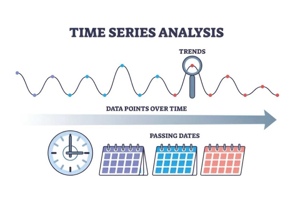
Time series analysis is one of the most widely used quantitative forecasting methods. It involves analyzing historical data points collected over time to identify trends, seasonal patterns, and cyclical fluctuations.

Moving Averages

Moving averages smooth out short-term fluctuations and highlight long-term trends. The simplest form is the Simple Moving Average (SMA), which calculates the average of a fixed number of past data points.

For example, let’s say you want to forecast monthly sales for a retail store. You have the following sales data for the past six months:

Month	Sales ($)
January	10,000
February	12,000
March	11,000
April	13,000
May	14,000
June	15,000

To calculate a 3-month moving average for July, you would take the average of April, May, and June:

$\text{SMA} = \frac{13,000 + 14,000 + 15,000}{3} = 14,000$

This suggests that sales for July are likely to be around $14,000.

Exponential Smoothing

Exponential smoothing is a more sophisticated time series method that assigns exponentially decreasing weights to past observations. The formula for exponential smoothing is:

$\hat{Y}_{t+1} = \alpha Y_t + (1 - \alpha) \hat{Y}_t$

Where:

• $\hat{Y}_{t+1}$ is the forecast for the next period.
• $Y_t$ is the actual value at time $t$.
• $\hat{Y}_t$ is the forecast for the current period.
• $\alpha$ is the smoothing factor (0 < $\alpha$ < 1).

Let’s use the same sales data to forecast July sales using exponential smoothing with $\alpha = 0.3$. Assume the forecast for June was $14,500.

$\hat{Y}_{July} = 0.3 \times 15,000 + (1 - 0.3) \times 14,500 = 4,500 + 10,150 = 14,650$

This method gives more weight to recent data, making it more responsive to changes.

2. Regression Analysis

Regression analysis is a powerful tool for understanding the relationship between variables. It’s particularly useful when you want to forecast a dependent variable based on one or more independent variables.

Simple Linear Regression

Simple linear regression models the relationship between two variables using a straight line. The equation for a simple linear regression is:

$Y = a + bX + \epsilon$

Where:

• $Y$ is the dependent variable.
• $X$ is the independent variable.
• $a$ is the intercept.
• $b$ is the slope.
• $\epsilon$ is the error term.

For example, suppose you want to forecast sales based on advertising spend. You have the following data:

Advertising Spend ($)	Sales ($)
1,000	10,000
2,000	15,000
3,000	20,000
4,000	25,000
5,000	30,000

Using regression analysis, you can estimate the relationship between advertising spend and sales. The slope ($b$) and intercept ($a$) can be calculated using the least squares method.

$b = \frac{n(\sum XY) - (\sum X)(\sum Y)}{n(\sum X^2) - (\sum X)^2}$ $a = \frac{\sum Y - b \sum X}{n}$

After performing the calculations, you might find that the regression equation is:

$Y = 5,000 + 5X$

This means that for every $1,000 increase in advertising spend, sales increase by $5,000.

3. ARIMA Models

ARIMA (AutoRegressive Integrated Moving Average) models are a class of statistical models used for time series forecasting. They combine autoregression (AR), differencing (I), and moving averages (MA) to capture complex patterns in data.

The general form of an ARIMA model is:

$\text{ARIMA}(p, d, q)$

Where:

• $p$ is the number of autoregressive terms.
• $d$ is the number of differencing operations.
• $q$ is the number of moving average terms.

For example, an ARIMA(1,1,1) model can be written as:

$(1 - \phi_1 B)(1 - B)Y_t = (1 + \theta_1 B)\epsilon_t$

Where:

• $B$ is the backshift operator.
• $\phi_1$ is the autoregressive parameter.
• $\theta_1$ is the moving average parameter.
• $\epsilon_t$ is the error term.

ARIMA models are highly flexible and can handle a wide range of time series data. However, they require careful parameter selection and validation.

Applications of Quantitative Forecasting

Quantitative forecasting has a wide range of applications across industries. Below, I’ll discuss some of the most common use cases.

1. Financial Markets

In financial markets, quantitative forecasting is used to predict stock prices, interest rates, and currency exchange rates. For example, hedge funds and investment banks use sophisticated models to identify trading opportunities and manage risk.

2. Supply Chain Management

Quantitative forecasting helps businesses optimize inventory levels, reduce costs, and improve customer satisfaction. For instance, retailers use demand forecasting models to ensure they have the right products in stock at the right time.

3. Economic Policy

Governments and central banks use quantitative forecasting to inform economic policy decisions. For example, the Federal Reserve uses econometric models to predict inflation and unemployment rates, which guide monetary policy.

4. Healthcare

In healthcare, quantitative forecasting is used to predict patient demand, allocate resources, and plan for emergencies. For example, hospitals use forecasting models to estimate the number of beds needed during flu season.

Challenges and Limitations

While quantitative forecasting is a powerful tool, it’s not without its challenges. One of the biggest limitations is the reliance on historical data. If the future deviates significantly from the past, quantitative models may produce inaccurate forecasts.

Another challenge is the complexity of some methods, such as ARIMA models. These models require a deep understanding of statistics and may not be accessible to all users.

Finally, quantitative forecasting often struggles to account for qualitative factors, such as changes in consumer behavior or geopolitical events. In these cases, combining quantitative and qualitative methods can produce more accurate results.

Conclusion

Mastering quantitative forecasting techniques is essential for anyone involved in financial planning, risk management, or decision-making. By understanding the methods, examples, and applications discussed in this article, you can make more informed predictions and drive better outcomes for your organization.