Demystifying Regression Analysis: Understanding Relationships in Data

Regression analysis is one of the most powerful tools in the world of data science, finance, and accounting. It helps us understand the relationships between variables and make predictions based on data. In this article, I will break down regression analysis into its core components, explain how it works, and show you how to apply it in real-world scenarios. Whether you’re a finance professional, an accountant, or someone curious about data, this guide will help you grasp the concepts with clarity and confidence.

What Is Regression Analysis?

At its heart, regression analysis is a statistical method that examines the relationship between a dependent variable and one or more independent variables. The goal is to model this relationship so we can predict the dependent variable based on the values of the independent variables. For example, in finance, we might use regression analysis to predict stock prices based on factors like interest rates, GDP growth, or company earnings.

The simplest form of regression is linear regression, where we assume a straight-line relationship between the variables. However, regression analysis can also handle more complex relationships, such as polynomial or logistic regression. I’ll explore these variations later in the article.

The Basics of Linear Regression

Let’s start with linear regression, the most straightforward and widely used form of regression analysis. In linear regression, we model the relationship between the dependent variable Y and the independent variable X using the equation:

Y = \beta_0 + \beta_1 X + \epsilon

Here:

• Y is the dependent variable we want to predict.
• X is the independent variable we use to make the prediction.
• \beta_0 is the y-intercept, representing the value of Y when X is zero.
• \beta_1 is the slope, indicating how much Y changes for a one-unit change in X.
• \epsilon is the error term, accounting for the variability in Y not explained by X.

Example: Predicting House Prices

Suppose I want to predict the price of a house based on its size in square feet. Here, the house price is the dependent variable Y, and the size is the independent variable X. Using historical data, I can estimate the values of \beta_0 and \beta_1 to create a predictive model.

Let’s say I find that \beta_0 = 50,000 and \beta_1 = 300. The regression equation becomes:

Y = 50,000 + 300X

If a house is 1,500 square feet, the predicted price would be:

Y = 50,000 + 300(1,500) = 500,000

This means the model predicts a house of 1,500 square feet would cost $500,000.

Assumptions of Linear Regression

For linear regression to provide accurate results, certain assumptions must hold true. These include:

1. Linearity: The relationship between the dependent and independent variables is linear.
2. Independence: Observations are independent of each other.
3. Homoscedasticity: The variance of the error terms is constant across all levels of the independent variables.
4. Normality: The error terms are normally distributed.
5. No Multicollinearity: Independent variables are not highly correlated with each other.

If these assumptions are violated, the regression model may produce unreliable results. I’ll discuss how to check for these assumptions later in the article.

Multiple Linear Regression

In many real-world scenarios, the dependent variable is influenced by more than one independent variable. For example, house prices might depend on size, location, and the number of bedrooms. In such cases, we use multiple linear regression, which extends the simple linear regression model to include multiple predictors.

The equation for multiple linear regression is:

Y = \beta_0 + \beta_1 X_1 + \beta_2 X_2 + \dots + \beta_n X_n + \epsilon

Here, X_1, X_2, \dots, X_n are the independent variables, and \beta_1, \beta_2, \dots, \beta_n are their respective coefficients.

Example: Predicting House Prices with Multiple Variables

Let’s expand the house price example to include the number of bedrooms and the crime rate in the neighborhood. The regression equation might look like this:

Y = 50,000 + 300X_1 + 20,000X_2 - 10,000X_3

Where:

• X_1 is the size in square feet.
• X_2 is the number of bedrooms.
• X_3 is the crime rate.

For a house with 1,500 square feet, 3 bedrooms, and a crime rate of 2, the predicted price would be:

Y = 50,000 + 300(1,500) + 20,000(3) - 10,000(2) = 550,000

This model predicts the house would cost $550,000.

Evaluating Regression Models

Once we build a regression model, we need to evaluate its performance. Key metrics include:

1. R-squared (R^2): Measures the proportion of variance in the dependent variable explained by the independent variables. An R^2 of 1 indicates a perfect fit, while 0 indicates no explanatory power.
2. Adjusted R-squared: Adjusts R^2 for the number of predictors in the model. It penalizes adding unnecessary variables.
3. Mean Squared Error (MSE): Measures the average squared difference between the predicted and actual values. Lower values indicate better fit.
4. P-values: Indicate the statistical significance of each predictor. A p-value less than 0.05 typically suggests the predictor is significant.

Example: Evaluating the House Price Model

Suppose the house price model has an R^2 of 0.85, meaning 85% of the variance in house prices is explained by the model. The p-values for size, bedrooms, and crime rate are all less than 0.05, indicating these variables are significant predictors. The MSE is 10,000, suggesting the model’s predictions are, on average, $10,000 off from the actual prices.

Common Pitfalls in Regression Analysis

While regression analysis is a powerful tool, it’s not without its challenges. Here are some common pitfalls to watch out for:

1. Overfitting: Including too many predictors can make the model fit the training data perfectly but perform poorly on new data. To avoid this, use techniques like cross-validation or regularization.
2. Multicollinearity: When independent variables are highly correlated, it can distort the coefficients and make the model unstable. Check for multicollinearity using the Variance Inflation Factor (VIF).
3. Outliers: Extreme values can skew the results. Identify and address outliers before building the model.
4. Nonlinear Relationships: If the relationship between variables is nonlinear, a linear regression model will fail to capture it. Consider using polynomial regression or other nonlinear methods.

Advanced Regression Techniques

While linear regression is a great starting point, many real-world problems require more advanced techniques. Here are a few worth exploring:

1. Polynomial Regression: Used when the relationship between variables is nonlinear. The regression equation includes higher-order terms, such as X^2 or X^3.
2. Logistic Regression: Used for binary classification problems, such as predicting whether a customer will churn or not.
3. Ridge and Lasso Regression: Regularization techniques that prevent overfitting by adding a penalty for large coefficients.
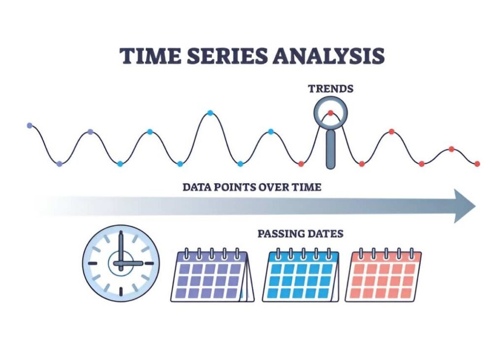
4. Time Series Regression: Used when data points are collected over time, such as stock prices or economic indicators.

Example: Polynomial Regression

Suppose the relationship between house prices and size is not linear but follows a curve. We can use polynomial regression to model this:

Y = \beta_0 + \beta_1 X + \beta_2 X^2 + \epsilon

If \beta_0 = 50,000, \beta_1 = 300, and \beta_2 = -0.1, the equation becomes:

Y = 50,000 + 300X - 0.1X^2

For a house of 1,500 square feet, the predicted price would be:

Y = 50,000 + 300(1,500) - 0.1(1,500)^2 = 425,000

This model predicts the house would cost $425,000.

Practical Applications in Finance and Accounting

Regression analysis has numerous applications in finance and accounting. Here are a few examples:

1. Risk Management: Predicting the likelihood of loan defaults based on borrower characteristics.
2. Portfolio Management: Estimating the relationship between stock returns and market indices.
3. Cost Accounting: Analyzing the relationship between production volume and costs.
4. Auditing: Identifying unusual patterns in financial data that may indicate fraud.

Example: Predicting Stock Returns

Suppose I want to predict the return of a stock based on the S&P 500 index. Using historical data, I can build a regression model:

Y = \beta_0 + \beta_1 X + \epsilon

Where:

• Y is the stock return.
• X is the S&P 500 return.

If \beta_0 = 0.02 and \beta_1 = 1.5, the equation becomes:

Y = 0.02 + 1.5X

If the S&P 500 return is 0.05, the predicted stock return would be:

Y = 0.02 + 1.5(0.05) = 0.095

This means the model predicts a 9.5% return for the stock.

Conclusion

Regression analysis is a versatile and powerful tool for understanding relationships in data. Whether you’re predicting house prices, analyzing stock returns, or managing costs, regression models can provide valuable insights. By mastering the basics and exploring advanced techniques, you can unlock the full potential of this method.